When I started out in statistics, fresh out of college, a general point of confusion was linear versus nonlinear regression modeling. It was easy enough to push a button and analyze data using statistical software, but how was I supposed to interpret the output? What were the mathematical and statistical techniques that the software was using in the background? It all seemed very black box.
In the spirit of the 2019 major league baseball postseason finally coming to an end, I thought it might be worthwhile to briefly touch on this topic (linear versus nonlinear regression modeling) using two common models and a rather simplistic set of baseball data. After providing this example (Part 1), I want to make some general comments regarding how statistical software fits models to your data and why nonlinear modeling can be confusing (Part 2).
In order to come up with a toy example for this post, I visited www.baseball-reference.com and downloaded 2019 regular season pitching game logs for Max Scherzer, ace pitcher for the Washington Nationals. From these game logs, I then selected games in which Scherzer was the starting pitcher and was assigned either a win or a loss (the “pitcher of record”). Here is a select portion of that dataset:
| Date | Team | Opponent | Decision | Hits Allowed | Strikeouts | |
|---|---|---|---|---|---|---|
| Mar 28 | WSN | NYM | L | 2 | 12 | |
| Apr 2 | WSN | PHI | L | 7 | 9 | |
| Apr 7 | WSN | @ | NYM | W | 8 | 7 |
| Apr 20 | WSN | @ | MIA | L | 11 | 9 |
| May 1 | WSN | STL | L | 8 | 8 | |
| May 11 | WSN | @ | LAD | W | 5 | 7 |
| May 17 | WSN | CHC | L | 6 | 8 | |
| Jun 2 | WSN | @ | CIN | W | 3 | 15 |
| Jun 8 | WSN | @ | SDP | W | 6 | 9 |
| Jun 14 | WSN | ARI | W | 3 | 10 | |
| Jun 19 | WSN | PHI | W | 4 | 10 | |
| Jun 25 | WSN | @ | MIA | W | 5 | 10 |
| Jun 30 | WSN | @ | DET | W | 4 | 14 |
| Jul 6 | WSN | KCR | W | 4 | 11 | |
| Sep 8 | WSN | @ | ATL | W | 2 | 9 |
| Sep 13 | WSN | ATL | L | 7 | 6 | |
| Sep 18 | WSN | @ | STL | L | 7 | 11 |
| Sep 24 | WSN | PHI | W | 5 | 10 |
Let’s say I want to ask two questions pertaining to Scherzer’s 2019 performance:
Q1: What’s the relationship between hits allowed and strikeouts?
Q2: What’s the relationship between hits allowed and win/loss decision?
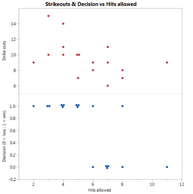
While these questions aren’t particularly important or relevant from a sabermetric standpoint, they do provide a platform for a side-by-side comparison of two basic regression models. Before we get into modeling, however, the respective data are plotted below. (I did drop Scherzer’s first outing from the dataset. I suppose you could justify this since it was his first game of the season and he was settling in to his rhythm for the year, but the only reason I did so was because it provides a better dataset for this illustration.)

When we look at the data as plotted we can make two observations, both of which are fairly intuitive:
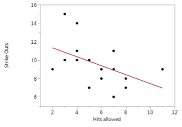
O1: Hits allowed and strikeouts are inversely related to one another. In other words, for any given game, if Scherzer gave up an abnormally high number of hits, then it looks like the total strikeouts for that game were lower than average. Contrapositively, for high strikeout games, it looks like he gave up fewer hits on average.
O2: When we use coded data for win/loss decision, where “1” corresponds to a win and “0” corresponds to a loss, we can also see from the above plot that wins correlate to games in which Scherzer allowed a relatively low number of hits allowed. Losses correspond to a relatively high number of hits allowed.
Ignoring the fact that both strikeouts and hits allowed are discrete numeric variables, we can address Q1 and Q2 using two regression models. (In this case I will assume they are continuous numeric variables. How variable type relates to model selection is a topic for another time.) The specific models we will use are:
M1: The simple linear regression model. We’ll use this to model strike outs.
M2: The simple logistic regression model. We’ll use this to model decision.
For both of these models, “simple” refers to the fact that we are using only one input or predictor variable. In this case, “hits allowed” is the sole input variable we are using to model either decision or strike outs.
Conceptually, I think M1 is pretty easy to visualize. We essentially have a quantitative response variable (strike outs) and want to model its relationship with another quantitative variable (hits allowed). Use of the term “linear” in M1 communicates that we are going to model this relationship with a straight line as shown below:

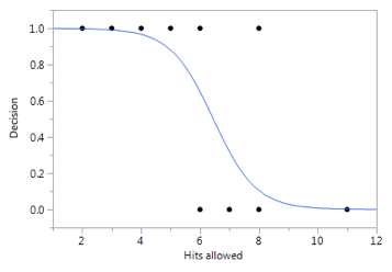
M2 is a basic nonlinear regression model that is commonly used for binary response variables. Rather than fitting a straight line through the data as in M1, M2 captures the step change relationship between decision and hits allowed using a nonlinear s-shaped curve:

M2 fits our intuition: as hits allowed increases, decision asymptotically approaches “loss.” As hits allowed decreases, decision asymptotically approaches “win.”
Since M1 is simply a straight line through our data, we can easily express this function without much thought:

Where  is the number of strikeouts for game i,
  is the intercept,
  is the slope term that relates hits allowed to strikeouts,
  is the number of hits allowed for game i, and
  is the error term. I’m using “S” superscripts to distinguish my strikeout model from my decision model.
M2 takes a little more effort. The logistic model I will use is

For M2 in particular (“logistic regression”), you’ll often hear people talk about a “link function.” Anytime we model data, we have choices to make: modeling choices that should be justified based on experience, statistical theory, or hopefully a little bit of both. Whenever we use logistic regression, we have options for expressing the exact nonlinear functional relationship between X and Y. For M2 as it is written above, I used a popular link function known as the logit link. For now, without going into all the details of how to interpret the M2 parameters, think of this as a model for estimating the probability of a “win” decision as highlighted in Figure 3.
Since we now have models that can be applied to our dataset, we can use software to come up with respective parameter estimates. I used JMP to analyze these data and came up with the following estimates:
For M1:  ;
; 
For M2:  ;
; 
We could then use these estimates to make predictions if we so desired. Suppose we watch a game in which Scherzer allows 7 hits. On average we might reasonably expect
12.302 – 0.486 7 = 8.9 strikeouts and a
 probability of being assigned a win*.
Having fit two rather simplistic regression models to our dataset, one linear and one nonlinear, in Part 2 I want to discuss some more general considerations. How are model estimates calculated? Does the type of model matter?
For now I’ll conclude by saying: go Nats!
*Assuming he is the pitcher of record. Like I said before, this particular example isn’t overly insightful in terms of its practicality.
In Part 1, I mentioned my early confusion regarding nonlinear versus linear regression modeling in terms of what goes on behind the scenes. How are these estimates calculated in the first place?
For any model you apply to a given dataset, linear models have the most historical mileage. They have been used since the dawn of statistics and employ rather basic mathematical/statistical assumptions for how variables relate to one another. As such, there is a wealth of statistical theory pertaining to linear modeling and the parameter estimates for linear models will typically have closed-form solutions (in other words, linear models are mathematically tractable). When JMP or any other statistical software package fits a linear model to your data, they are using matrix algebra (aka linear algebra) to come up with a solution.
The price you pay for using a linear model is that it may not adequately capture intra-variable relationships and, as such, may be of limited use in the real world.
For nonlinear models, on the other hand, it will almost always be necessary to rely on numerical methods that use computational algorithms to come up with model parameter estimates. Very rarely will a closed-form solution exist for your model. Assuming you have selected an appropriate nonlinear model for your data, you will often have more choices to make in terms of how the parameters for this nonlinear model are estimated. And for life in general, you could make a strong argument that too many choices often leads to confusion.
When a statistical software package fits a nonlinear model to your data (or if you are writing custom code), then two methods will usually be used to come up with parameter estimates:
- Least squares. This method takes the data you have on hand and comes up with parameter estimates that will minimize total squared distances between Y as observed and Y as predicted. For this approach, you only need the deterministic nonlinear functional relationship between X and Y.
- Maximum likelihood. For this method, you’ll need to derive the overall likelihood function for your dataset. In contrast to A, you will need the stochastic distributional relationship between X and Y (the probability density function aka PDF).
To complicate matters further, it is often not a simple matter of merely minimizing A or maximizing B to come up with parameter estimates. Depending on the functional expression of your model, it often makes computational sense to rely on partial derivatives (normal equations) or apply a logarithmic transformation. If you are relying on software, then these decisions are made for you. If you are writing custom code, then this is where experience and a basic understanding of statistical computation are your friends.
And, unfortunately, there are still more choices to make!
Nonlinear optimization based on either A. or B. always poses the risk of coming up with suboptimal parameter estimates. To avoid this it is often necessary to make several choices regarding how you will search the parameter space and, specifically, which parameter values you will use as initial estimates. This will help us avoid minima/maxima that are local instead of global.
And, to cap it all off, you still have to decide which optimization algorithm you will use to actually minimize A. or maximize B. Whew!
If you are using fairly standard models and if you rely on out-of-the-box software, then you probably don’t need to spend too much time thinking about all of the above. If you’re like me, however, it’s intellectually satisfying to have at least a rudimentary understanding of what is going on below the surface. And as you progress within the field of data science, this understanding is absolutely crucial. You can probably carve out a career simply using software to crunch some numbers, but understanding the “why” is what makes the difference between a job that pays the bills and one that is truly satisfying.